AI accelerated FEM solvers: Improving convergence with better initialisation

Numerical simulation is the backbone of modern engineering. From stress analysis to electromagnetics, methods such as finite element modelling (FEM) help engineers predict how designs will behave long before anything is built. Precision, however, doesn't come for free, and there is typically a trade-off between prediction accuracy and computational cost. On one end of the spectrum, numerical methods such as FEM come with theoretical guarantees and are often the gold standard, but their computational burden and their licensing costs can make them a bottleneck in the design process. On the other end, surrogate models can provide approximate solutions at a fraction of the cost, but the surrogate prediction errors tend to compound when used in an optimisation context.

This blog post focusses on electric motor design, where evaluating a single motor design requires hundreds of nonlinear electromagnetic simulations. At the scale of modern optimisation workflows, these simulations dominate compute costs and their surrogate model counterparts are often deemed too inaccurate to be used as a replacement. We investigate here a hybrid approach where a deep learning model is used to initialise a FEM solver, and show that it reduces simulation time by up to 30% while retaining the accuracy and guarantees of finite element analysis.

The work builds on a foundation that Monumo has spent years developing: a proprietary simulation platform capable of solving millions of motor operating points per day, a large corpus of synthetic physics data generated from those simulations, and machine learning models designed specifically for mesh-based engineering problems.

1Electromagnetic solvers

The key metrics that characterise the electromagnetic behaviour and performance of a motor - flux linkage, torque, back-EMF, core losses - can be derived from the magnetic flux density $\mathbf{B}(x, y, z, t)$ which is a vector-valued function over space and time. In the context of electric motors, Maxwell's equations boil down to:

where the reluctivity $\nu$ describes how strongly the material opposes the creation of magnetic flux and $\mathbf{J}$ is the current density. Since the divergence of a curl is always zero, a convenient reparametrisation that satisfies the divergence free constraint by construction is to write $\mathbf{B} = \nabla \times \mathbf{A}$ where $\mathbf{A}$ is the magnetic vector potential. Furthermore, the magnetic field $\mathbf{B}$ tends to be confined to the $(x, y)$ plane for radial flux machines, so out of the three components of $\mathbf{A}$ it is reasonable to assume that only the last one $a_z(x,y)$ is non-zero. In the end, Maxwell's equation collapses to one scalar equation over the cross-section:

where $j_z$ captures both the axial current density imposed in the windings and the permanent magnet contributions.

Given the complexity of electric motor geometries, there is no analytic solution to this equation, and one must use numerical methods to obtain a solution. The finite element method turns this PDE into algebra: the cross-section is meshed into triangles, $a_z$ is approximated by local basis functions $\varphi^{(i)}$ attached to the $d$ nodes of a mesh,

and the projection of eq. (1) onto those basis functions yields one algebraic equation per node. These equations can be assembled into a system of $d$ equations in $d$ unknowns

where $K$ is the stiffness matrix, $u$ is the vector of nodal values of $a_z$, and $J$ is the vector of currents at nodes. We'll skip the details here of how the system is modified to account for the boundary conditions but simply mention that Mortar boundary conditions are used to account for the angular periodicity and for stitching together the non-conformal rotor and stator meshes.

If $K$ does not depend on $u$, the solution $u = K^{-1}J$ can be obtained with a direct linear solver. The tricky part comes from the iron, for which $\nu$ isn't a constant. Indeed, the soft-magnetic steel in the rotor and stator saturates: its reluctivity rises steeply once the local flux density exceeds roughly $1.5$-$2\,$Teslas, so $\nu$ and $K$ depend on the very field being solved for. The assembled finite element equations therefore form a nonlinear system

To solve such systems for $u$, Newton-Raphson uses an iterative procedure where an initial guess, such as $u_0 = 0$, is sequentially improved by reducing the residual error:

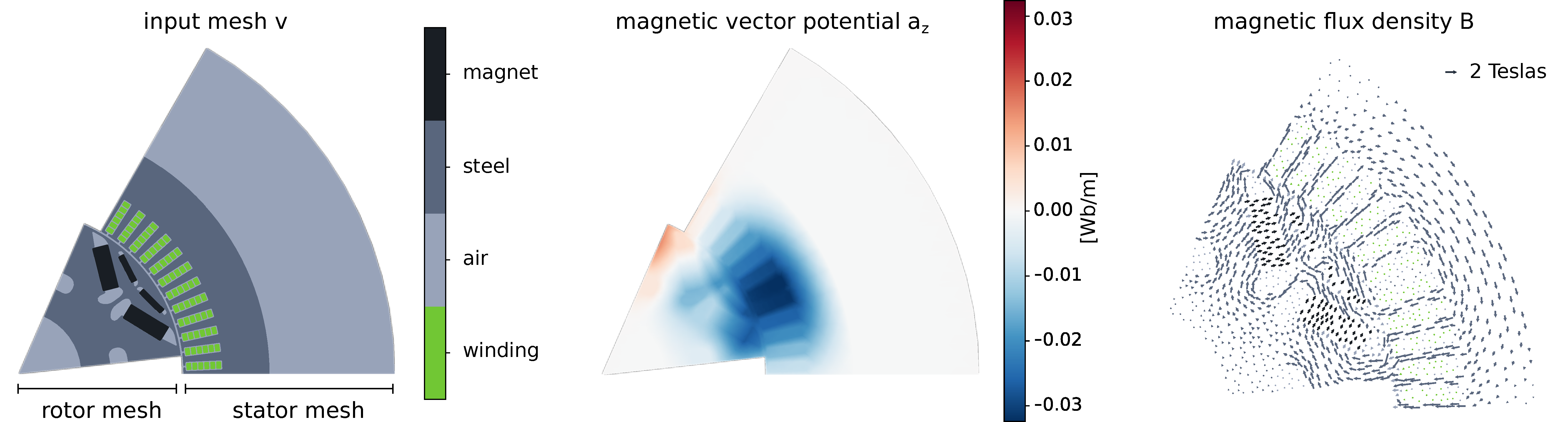
for vector-valued residual $R_n = K(u_{n}) u_{n} - J$ and tangent matrix $P_n = \nabla R_n$. After several iterations, the algorithm converges to the solution and we obtain a field as shown in Figure 1 (magnetic fluxes are spatially subsampled for exposition).

As one may expect, the number of iterations $N$ required to achieve convergence depends strongly on the quality of the initial guess $u_0$.

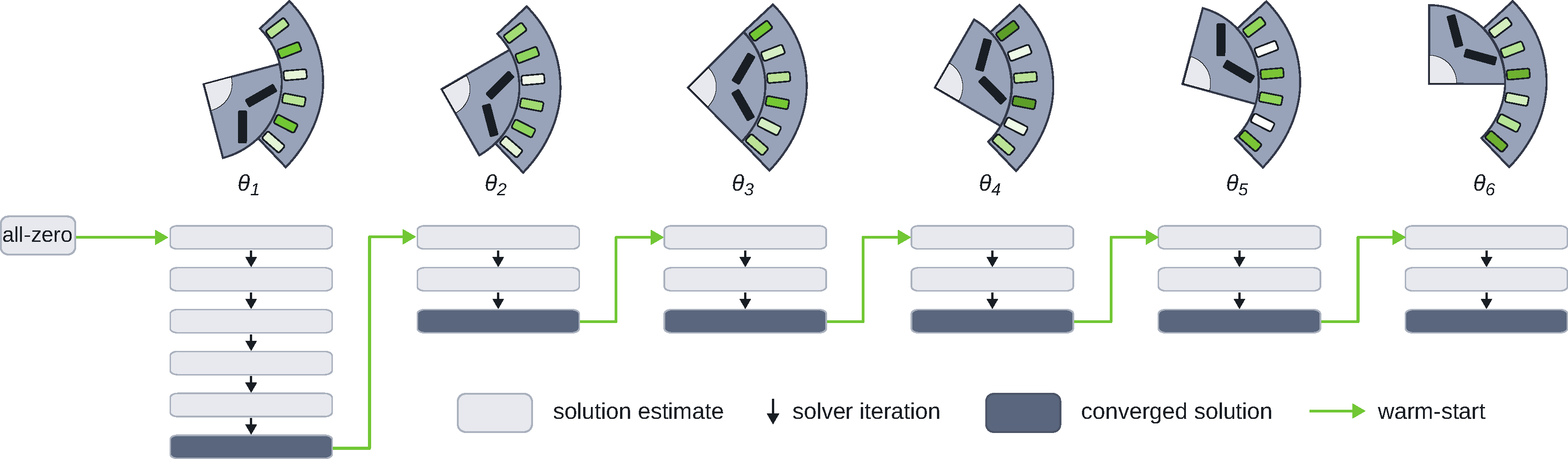
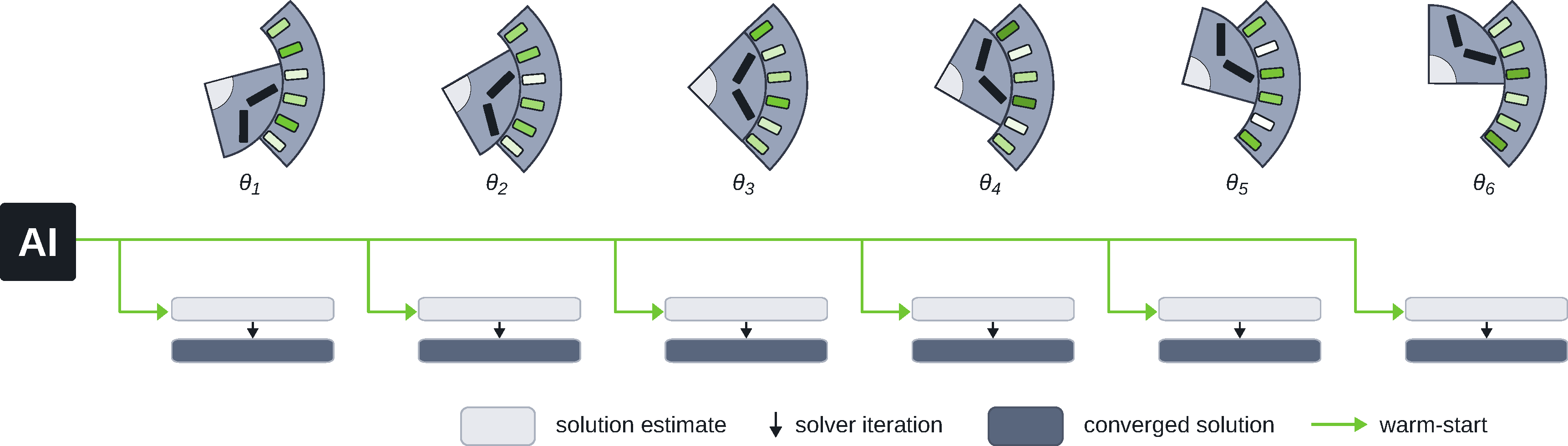
Since evaluating a motor's performance requires several hundred simulations (combinations of tens of rotor positions and waveforms), simulation engineers have long exploited shared structure between these repeated simulations to minimise overall computational costs. A common strategy to accelerate convergence is to warm start the solve with an already calculated solution. For example, when solving for $a_z$ at a given rotor angle $\theta_k$, using an existing solution at a nearby rotor angle as initialisation is a much better starting point than $u_0 = 0$. This is commonly implemented in FEM software, where the solution at $\theta_{k-1}$ is used to initialise the $\theta_{k}$ solve as depicted in Figure 2. In practice, this simple procedure can halve the number of iterations required.

In the next sections, we will see that convergence can be achieved even faster by initialising the solver with the predictions of a deep learning model.

2Foundation models as FEM surrogates

At Monumo, we built a platform that allows us to solve millions of electromagnetic problems per day. This high-throughput system supports our motor optimisation workflow and we also use it to collect large synthetic datasets for training deep learning models. In a nutshell, our aim is to build physics foundation models that can be used as a drop-in replacement for FEM solvers. Our models $f$ take meshed geometry $v$ as inputs and aim at predicting the magnetic field: $f(v) \approx u_N$.

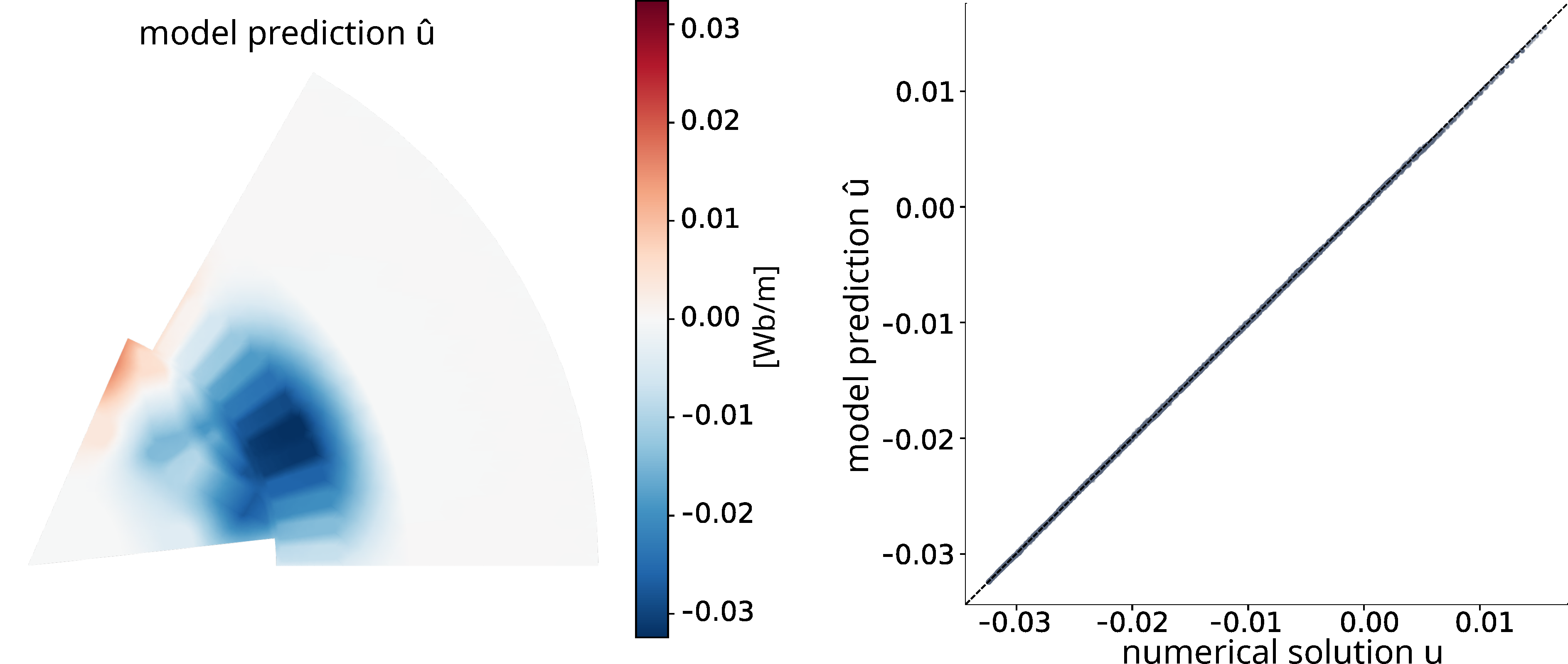
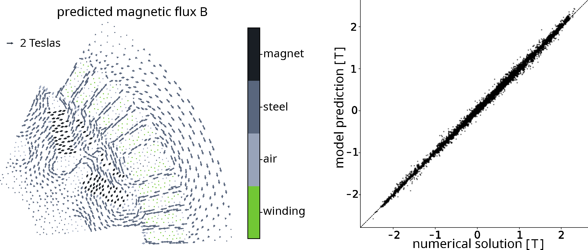
After experimenting with many different architectures, we found that models from the neural operator literature, with architectures that scale linearly in the number of nodes, offer a great cost vs accuracy trade-off. Indeed, those models can accurately predict the $a_z$ and $\mathbf{B}$ fields (Figures 3, 4) while offering orders of magnitude speed-ups compared to FEM solvers. However, various downstream tasks require different levels of prediction accuracy and, depending on the task at hand, these models may or may not be precise enough to replace the FEM solver. Here, we focus on the use-case where accuracy is paramount and show that even in this demanding setting deep learning models can accelerate FEM solvers while preserving all their guarantees. A follow-up blog-post will be dedicated to the models themselves and their potential to replace numerical solvers.

3AI accelerated solvers

We now have all the ingredients required to make an AI accelerated FEM solver. As often with ML models, we can make multiple predictions at once by batching together the set of designs we want to propagate through the model. In our case, this means computing the $a_z$ field for various rotor positions and current densities in the windings in a single forward pass. As illustrated in Figure 5, the prediction of the electromagnetic AI model can warm start the solvers by setting $u_0(v, \theta_k) = \hat u(v, \theta_k)$ before applying Newton-Raphson iterations until convergence.

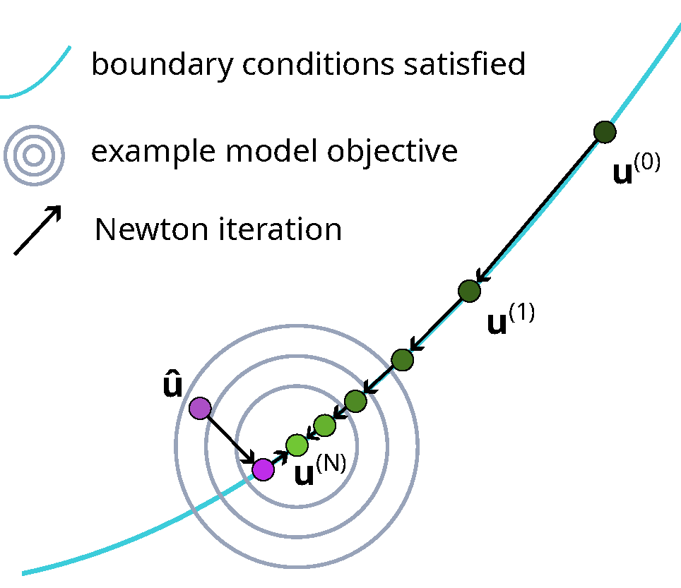
A key benefit from the Newton iteration is that it projects the model predictions $\hat u$ onto the boundary conditions even if the model output itself does not satisfy them. As shown schematically in Figure 6, this means that the prediction errors at the boundaries disappear in a single Newton-Raphson step.

That leaves the question of what loss function should be considered to train the physics AI models. When used as electromagnetic FEM substitutes, it makes sense for them to provide accurate predictions of the $a_z$ and $\mathbf{B}$ fields, so the loss function should be based on these quantities. In the context of solver initialisation, predicting fields well is less about absolute accuracy, and more about making errors that can easily be corrected by a small number of Newton-Raphson iterations. To achieve this, we experimented with fine-tuning our physics AI models with a "Newton-in-the-loop" loss function, where one step of (differentiable) Newton-Raphson correction is applied during training before computing the loss.

4Results and outlook

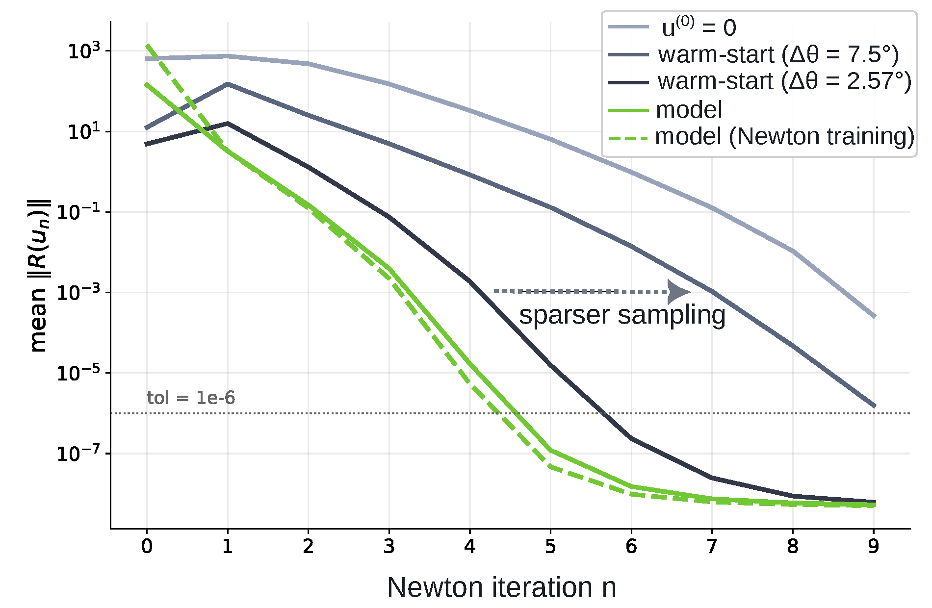
The comparison of the solver residuals as a function of the number of steps is shown in Figure 7. A few things stand out:

• Initialising $u_{0}=0$ results in residuals that are about an order of magnitude larger than the warm-start baselines, and requires the most steps to converge.
• The performance of a warm start re-using previous solutions depends on how similar the two angles are. For a finely discretised electrical period (35 time points), the difference between two consecutive angles is small ($\Delta \theta = 2.57\,\mathrm{deg}$) and the solver converges in 2/3 of the steps compared to a coarser discretisation (12 time steps, $\Delta \theta = 7.5\,\mathrm{deg}$). As differences in rotor angle $\Delta\theta$ between consecutive solves increase with sparser sampling within the drive cycle, it degrades towards the naive $u_{0} = 0$.
• Although the ML initialised solver starts with a larger residual, they converge at a favourable rate compared to all other methods. Note that their performance does not depend on the time sampling density so they have a larger edge when time discretisation is coarse.
• The Newton-in-the-loop fine tuning does not provide a substantial benefit compared to the AI physics model. Since the loss function here evaluates model outputs only after the first Newton iteration, it has the worst field prediction accuracy at $n=0$ but makes it up by making more progress in the first iteration.

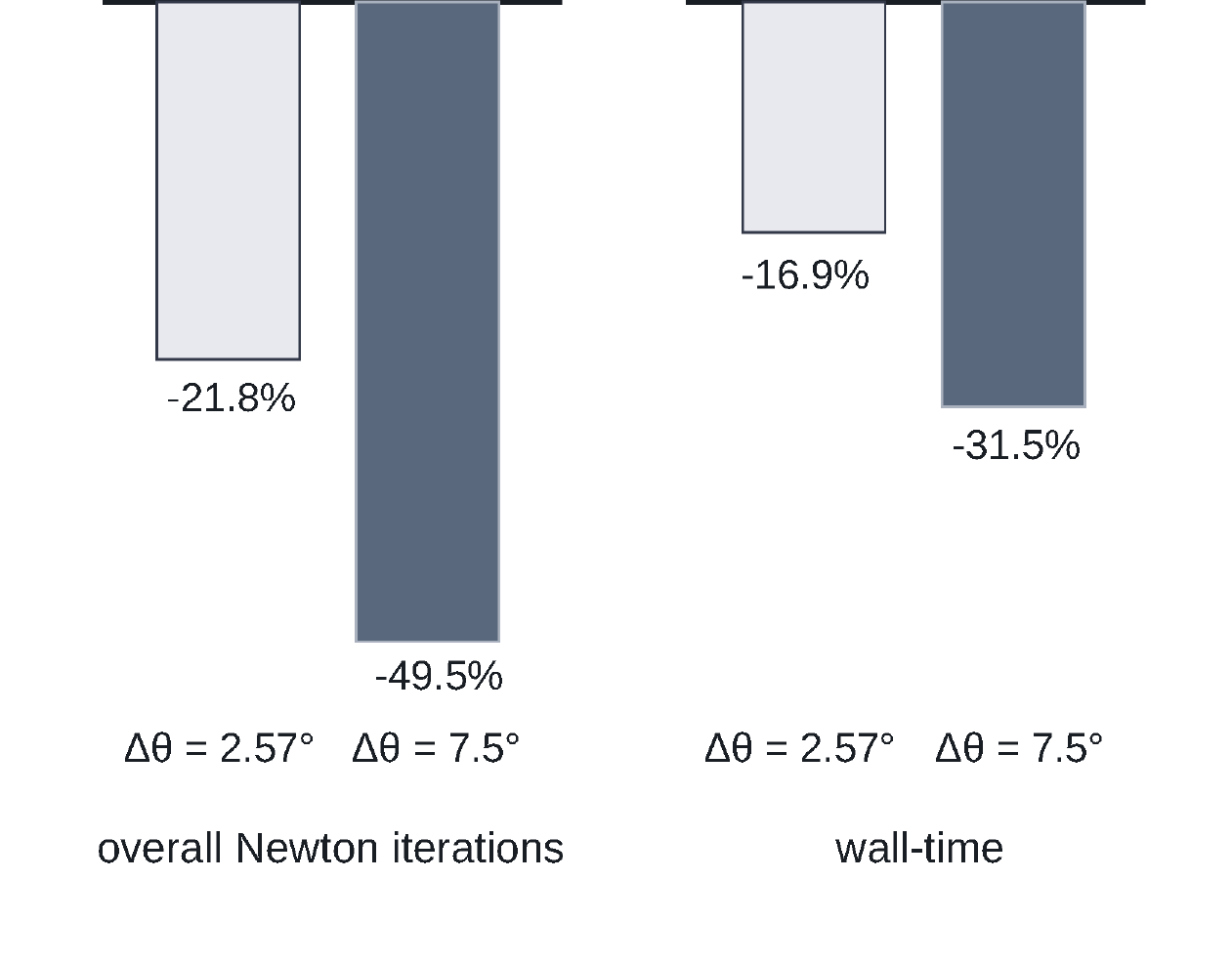
Finally, we compare the number of Newton iterations required to reach convergence as well as the associated wall-clock time in Figure 8. As expected, the amount of acceleration provided by AI depends on how strong the baseline is and hence on how finely time is discretised. Even in the case where the fine time discretisation is favourable to the baseline, we find that the AI initialisation can reduce compute time by 15%, and this saving doubles for coarser time discretisations.

The broader lesson is that when accuracy and theoretical guarantees matter most, AI cannot yet fully replace numerical solvers. Used in the right place, it can however work alongside classical numerical methods to reduce their computational cost while preserving the guarantees that make them so valuable in the first place.

For motor design, this means faster evaluation of candidate geometries, drive cycles, and operating points without giving up the precision needed for reliable engineering decisions. More broadly, the same approach opens the door to AI accelerated simulation across other physics domains, from thermal analysis to structural and contact mechanics. At Monumo, this is central to how we think about physics AI: not as a shortcut but as a way to make high-fidelity physics available earlier, faster, and at greater scale.